#30DayMapChallenge Day 10: Prompting only

Day 10 of the #30DayMapChallenge 2026.

Prompting only — For this map, make AI work for its money and produce something from start to finish in a chat window or on the command line.

This theme is a little moot for me. Every map so far this month has been prompt only. I have typed a question into MapAI, and it has found the data, written the SQL, run the analysis, styled the layers and written up the answer. Nine days, nine maps, no desktop GIS.

So the interesting question isn’t whether AI can make a map from a prompt. It clearly can. The question is: how do you know the map is right?

For Day 10 I am not making a new map. Instead I am taking yesterday’s map apart, to show what sits underneath the answer, and why that matters more than the answer itself.

The question

This is the Day 9 prompt, word for word:

Urban–rural transect: Sydney CBD to Lithgow.

1. Draw a straight line from Sydney Town Hall west to Lithgow town centre.
2. Select every SA2 (ASGS Edition 3) that the line passes through, and give each one its distance in km from Town Hall, measured along the line to where the line enters the SA2.
3. For each of those SA2s, get: 2025 ABS ERP and population density (people per km²), median age and median weekly household income (2021 Census), and the Modified Monash Model class.

Output 2 layers:

1. The transect SA2s as a choropleth of population density, using a log scale, dark for dense and light for sparse.
2. The transect line as a thin white line.

Tooltips: SA2 name, distance from CBD (km), population density, median age, median household income, MMM class.

Tell me, in a table ordered by distance from the CBD: each SA2’s distance, density, median age, income and MMM class. Then tell me where the city ends (the first SA2 below 100 people per km²), where the MMM class first changes from metropolitan, and how age and income change from the CBD to Lithgow. List your assumptions.

The answer

MapAI drew a 103.34 km line that crosses 32 SA2s, and summed it up in four findings:

• The city ends at Yarramundi - Londonderry, the first SA2 below 100 people per km², 55.22 km from Town Hall.
• The country begins at Blue Mountains - North, 57.92 km out, where the MMM class changes from Metropolitan straight to Small rural towns.
• Median age rises from 37 in the CBD to 46 in Lithgow, peaking at 61 in Blue Mountains - North.
• Median weekly household income falls from $2,457 to $1,088, down $1,369 or 55.7%.

That is a clean, confident, quotable answer. It is also exactly the kind of answer you should not trust on its own.

Not because it is wrong, but because nothing in those four bullets tells you how it was reached. Where exactly is “Sydney Town Hall”? Which income: household, family or personal? Which year’s boundaries? What happens when an SA2 sits across two remoteness classes? A wrong answer to any of these would still produce four clean, confident bullets.

AI answers have one tone of voice. They sound the same when they are right as when they are wrong. The only way to tell the difference is to look underneath.

What sits underneath

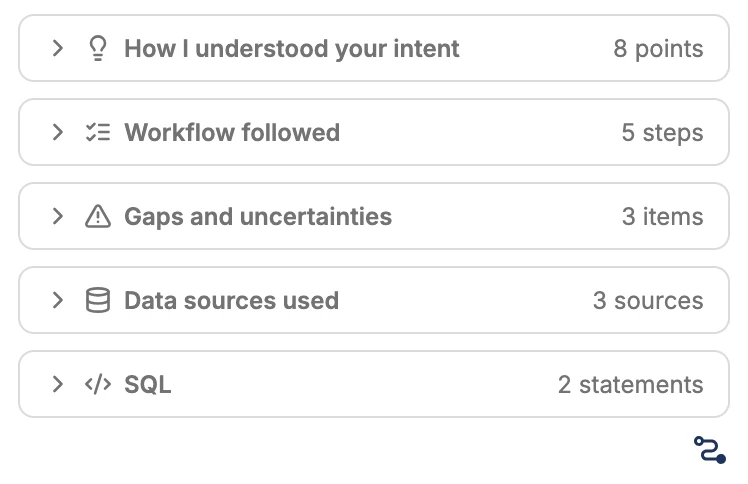
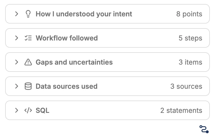
Every MapAI answer comes with an evidence trail: five panels that sit below the answer and open on demand. Here is what each one showed for Day 9, and why it is there.

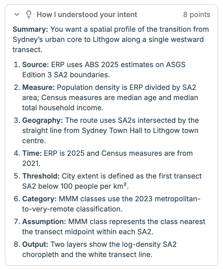
1. How I understood your intent

Summary: You want a spatial profile of the transition from Sydney’s urban core to Lithgow along a single westward transect.

Then eight points: the source (ABS 2025 ERP on ASGS Edition 3 SA2s), the measure (density is ERP divided by SA2 area; median age and median total household income), the geography, the time (ERP is 2025, Census is 2021), the threshold (first SA2 below 100 people per km²), the category (MMM 2023), one assumption and the output.

This is the first thing to check, before any number. If the restated question is wrong, every number after it is an answer to a different question. It is the same as a colleague reading your brief back to you before they start: cheap, fast, and it catches most misunderstandings at the door.

Two things here are worth noticing. It says median total household income, so the income question is settled in writing, not silently. And it says, in plain words, that the ERP is 2025 and the Census measures are 2021. That mismatch was in my prompt, and the trail makes sure nobody forgets it when they quote the result.

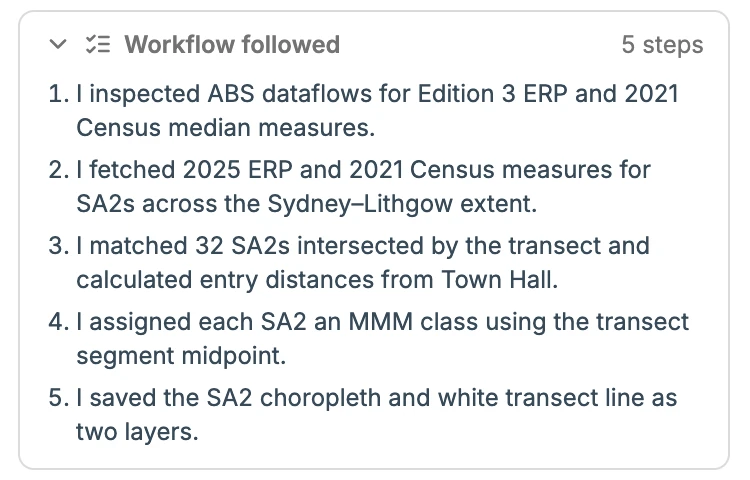
2. Workflow followed

Five steps:

1. Inspected the ABS dataflows for Edition 3 ERP and 2021 Census median measures.
2. Fetched 2025 ERP and 2021 Census measures for SA2s across the Sydney–Lithgow extent.
3. Matched the 32 SA2s intersected by the transect and calculated entry distances from Town Hall.
4. Assigned each SA2 an MMM class using the transect segment midpoint.
5. Saved the choropleth and the white transect line as two layers.

The workflow is the order of operations. It tells you that MapAI went to the ABS Data API for the population and Census figures rather than using something it already had, and that it only fetched SA2s around the line. Step 4 is the one to note: remoteness is decided at one point per SA2, which matters for the big SA2s further west.

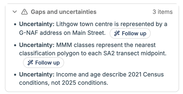
3. Gaps and uncertainties

MapAI flagged three:

• Lithgow town centre is represented by a G-NAF address on Main Street.
• MMM classes represent the nearest classification polygon to each SA2’s transect midpoint.
• Income and age describe 2021 conditions, not 2025.

This is the most important panel, and the one most tools leave out. Every analysis makes judgement calls. The difference is whether they are written down.

None of these three is a mistake. They are choices a GIS analyst would also have to make, and the panel says what was chosen so that you can disagree with it. Two of them come with a Follow up button, so the next question, “use the Lithgow SA2 centroid instead” or “show me every MMM class each SA2 touches”, is one click away.

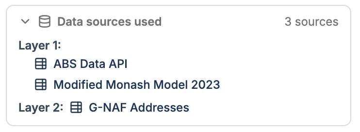
4. Data sources used

• Layer 1: ABS Data API and the Modified Monash Model 2023.
• Layer 2: G-NAF Addresses.

This is the bibliography. Read with the assumptions, it is also where the two ends of the line come from: Sydney Town Hall is the G-NAF point for 483 George Street, and Lithgow town centre is 19A Main Street. That one detail would never fit in a four-bullet answer, but it decides every distance on the map. Move either end and every SA2’s distance, and possibly the list of SA2s itself, changes.

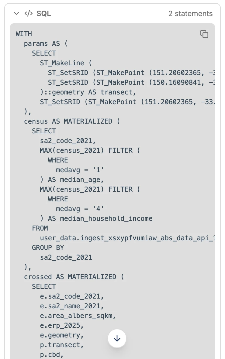
5. SQL

Two statements: one that builds the 32 SA2s with all their attributes, and one that draws the line. This is the part that turns “trust me” into “check me”. Everything else in the trail is MapAI’s own description of what it did. The SQL is what it did, and anyone who knows PostGIS can read it, rerun it or change it.

Reading the SQL

I read the main statement end to end. Here is what it confirms, and what it shows that the summary does not.

The two ends of the line are hard-coded, so there is no doubt about where “Town Hall” and “Lithgow” are:

ST_MakeLine (
  ST_SetSRID (ST_MakePoint (151.20602365, -33.87318490), 4326),
  ST_SetSRID (ST_MakePoint (150.16090841, -33.48031097), 4326)
)::geometry AS transect

The Census measures come from one ABS table, picked out by code:

MAX(census_2021) FILTER (WHERE medavg = '1') AS median_age,
MAX(census_2021) FILTER (WHERE medavg = '4') AS median_household_income

This is the single most useful line to check. MapAI has decided that code 1 means median age and code 4 means median household income. If it had picked the wrong code, the map would show personal income or family income, and nothing in the answer would look wrong. With the SQL in hand, it takes a minute to look the codes up in the ABS dataflow and confirm.

The one-metre rule from the assumptions is really in the code:

AND ST_Length (ST_Intersection (e.geometry, p.transect)::geography) > 1

That stops an SA2 that the line only clips at a corner from making the list. The stated assumption and the code agree, which is exactly what you want to see.

The distances are where the line first crosses each SA2’s boundary, as a fraction of the line, times the line’s total length. The SA2 that contains Town Hall is set to zero:

CASE
  WHEN ST_Covers (x.geometry, x.cbd) THEN 0.0
  ELSE (
    SELECT MIN(ST_LineLocatePoint (x.transect, d.geom))
    FROM ST_DumpPoints (ST_CollectionExtract (x.boundary_hits, 1)) d
  )
END AS entry_fraction

Reading this closely shows a small detail the assumptions gloss over. The total length is measured on the globe, but the fraction along the line is measured on a flat longitude-latitude grid. Over a 103 km line running mostly east–west, the difference is tiny and would not move any finding. But it is the kind of thing you can only see in the code, and on a much longer line you would want to know about it.

The remoteness class is the class of whichever MMM polygon is nearest to a single point: halfway between where the line enters and leaves each SA2.

ORDER BY ST_Distance (mm.geometry, w.transect_midpoint_7845)
LIMIT 1

So an SA2 that is half Metropolitan and half Small rural town gets just one label, from that one point. That is the second item in the gaps panel, now visible in code. It is a reasonable choice for a transect, but it means the “MMM changes at 57.92 km” finding is really “the class at the middle of Blue Mountains - North’s stretch of the line is Small rural towns”.

Missing data stays visible. The Census figures are joined with a LEFT JOIN, so an SA2 with no Census data would show up with a blank rather than quietly drop off the map.

None of this changes the Day 9 findings. That is the point: I can now say they hold, and say why, instead of hoping.

Why traceability matters

1. Confidence is not evidence. An AI answer reads the same whether it is right or wrong. The trail is what separates the two.

2. Every analysis is full of choices. Which point is “the town centre”? Which income? What counts as “passes through”? Without a trail, those choices are made silently, and you inherit them without knowing. With one, they are written down, and you can challenge them.

3. Numbers end up in reports. “Median household income falls 55.7% from the CBD to Lithgow” is exactly the kind of sentence that ends up in a council report or a funding application. Somebody will eventually ask where it came from. “The AI said so” is not an answer. “2021 Census median total household income, ABS Data API, SA2s crossed by a line from 483 George Street to 19A Main Street, and here is the SQL” is.

4. It makes the work repeatable. When the 2026 Census comes out, I don’t have to remember what I did. The SQL is there. Change the table and run it again.

5. It makes the next question better. Reading the gaps panel is how I knew to ask about the MMM rule. The trail doesn’t just justify the answer; it shows you where to push.

6. It is how a GIS analyst already works. Nobody experienced hands over a map without being able to say what data went into it and how. Traceability is not a new requirement invented for AI. It is the old standard, applied to a new tool.

What traceability doesn’t do

It doesn’t make the answer right. It makes it checkable, and checking still takes a person who knows what to look for.

It also can’t fix a vague question. If I had asked for “the population of each SA2” when I meant density, the trail would faithfully document a correct answer to the wrong question. The intent panel helps, because it says back what was understood, but you still have to read it.

And most of the trail is MapAI’s own account of itself. The intent, workflow and gaps panels are descriptions. The SQL is the part you can check independently, which is why it is worth having even if you only read the parts that matter.

The live map

You can explore the Day 9 map that this trail belongs to here: 09 Urban Rural - Sydney to Lithgow.

What I noticed

The Day 9 answer took MapAI 526 seconds, 32 tool calls and about 200 credits. What came back was four bullets and seven assumptions on top, and 8 intent points, 5 workflow steps, 3 uncertainties, 3 data sources and 2 SQL statements underneath.

That ratio is the point. The answer is what you quote; the trail is what lets you quote it. The AI does the fetching, joining and geometry, and the trail hands the judging back to the person.

The trail, panel by panel

Swipe or scroll sideways through the six screenshots.

Day 10 done. Tomorrow: sound.

#30DayMapChallenge #mapai #madewithmapai