#30DayMapChallenge Day 11: Senses: Sound

Day 11 of the #30DayMapChallenge 2026.

Senses: Sound — How do you hear something? How do you map a soundscape? Noise pollution mapped?

Sydney is getting a second airport. Western Sydney International, at Badgerys Creek, will put a new set of flight paths over the farms, villages and growing suburbs of the Western Parkland City. The planning system already maps how loud it is expected to be on the ground.

So for Day 11 I asked MapAI two short questions: where is the airport noise, and whose homes are in it?

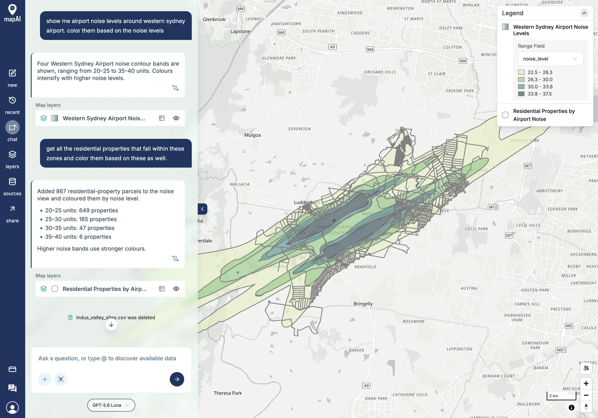
MapAI showing Western Sydney International Airport's noise contours as long bands stretching south-west to north-east along the runway, shaded from pale green for the 20–25 band to dark grey-blue for the 35–40 band, with property parcels outlined on top, and a chat panel listing 867 properties by noise band

The prompts

After yesterday’s long, carefully specified prompt, this one went the other way: two casual turns, written the way anyone would type them.

show me airport noise levels around western sydney airport. color them based on the noise levels

get all the residential properties that fall within these zones and color them based on these as well.

What MapAI found

Four noise bands, from 20–25 up to 35–40 units, running out from both ends of the runway in the long cigar shapes that flight paths make on the ground.

867 properties inside them:

Noise band	Properties
20–25 units	649
25–30 units	165
30–35 units	47
35–40 units	6

Three in every four are in the quietest band. But 218 are at 25 units or more, and 6 sit in the loudest band, right under the runway ends.

What MapAI did

By the numbers, both turns together took:

16 tool calls
About 5 minutes 50 seconds (350 seconds) from first prompt to finished map
About 100 credits

Here is its evidence trail, in its own words where possible.

How it understood the question

For the noise layer:

Source: the uploaded Airport Noise dataset.
Measure: airport noise contour units.
Geography: Western Sydney Airport, read as the Western Parkland City airport contours.
Assumption: each five-unit noise range represented by its midpoint, so 20–25 becomes 22.5, for graduated colouring.

For the properties:

Source: the Airport Noise and Properties datasets combined.
Category: freehold parcels with a primary address used as a stand-in for residential.
Assumption: a property touching more than one contour gets the highest band.

The workflow

Checked the noise dataset’s geometry and noise-range attributes.
Selected the four Western Parkland City contours and turned each range into a midpoint.
Checked the property schema and found no residential land-use field.
Filtered to freehold, primary-address parcels whose centre falls inside a contour.
Kept each parcel’s highest band and saved 867 properties as a coloured layer.

The data

The contours come from the planning layer “Australian Noise Exposure Concept (units)” under the State Environmental Planning Policy (Precincts—Western Parkland City) 2021. The properties come from MapAI’s base property data.

The SQL

Turning a text range like 25 - 30 into a number to colour by is a neat one-liner:

ROUND(
  (
    split_part(anef_code, ' - ', 1)::numeric + split_part(anef_code, ' - ', 2)::numeric
  ) / 2,
  1
) AS noise_level

And the “highest band wins” rule is a window function:

ROW_NUMBER() OVER (
  PARTITION BY p.id
  ORDER BY n.noise_level DESC
) AS zone_rank

Gaps and uncertainties

MapAI flagged three across the two turns:

Each noise range is drawn by its midpoint. Fine for colour, but the bands are ranges, not exact levels.
There is no residential land-use field in the property data, so freehold parcels with a primary address stand in for homes.
121 overlapping contour matches were resolved by keeping each property’s highest band.

You can explore the live map here: 11 Sound - Western Sydney Airport.

What I noticed

The contours are beautiful in an unsettling way. Two long bands follow the runway out to the south-west and north-east, and the darkest parts sit almost entirely inside the airport site. The pale 20–25 band is what reaches the neighbours: Luddenham, Badgerys Creek, Kemps Creek and the rural lots around them.

Two things in the trail are worth reading closely, which is exactly what yesterday’s post was about.

First, this is a concept, not a forecast. The planning layer is called the Australian Noise Exposure Concept, a planning layer, rather than the Australian Noise Exposure Forecast (ANEF) that airports use for their endorsed noise forecasts. The SQL column is still called anef_code, so the name in the data and the name of the layer don’t quite agree.

Second, the property count looks like a floor, not a total. The SQL only searches for properties inside a fixed box:

ST_MakeEnvelope (150.68, -33.93, 150.80, -33.83, 4326)

On the map, the outer band runs further than that: north-east past Kemps Creek towards Horsley Park, and south-west past Greendale. If I am reading that right, properties at both tails of the contours were never tested, so the real number is likely to be higher than 867. That is not in the gaps panel; it only shows up in the SQL. A follow-up asking MapAI to use the contours themselves as the search area would settle it.

For context, the Australian Standard for building near airports (AS 2021) treats 20–25 units as “conditionally acceptable” for houses and anything above 25 as “unacceptable”. That puts the 218 properties at 25 units and up in a different category from the other 649. The “residential” label is a proxy too, so some of the 867 will be sheds, farm lots or vacant land rather than homes.

Still, two casual sentences produced a map of what the new airport will sound like on the ground, and a list of the parcels under it, in under six minutes. And the trail was detailed enough to show where to push next.

Day 11 done. Tomorrow: power.

#30DayMapChallenge #mapai #madewithmapai